Merriam-Webster defines ageism as “prejudice or discrimination against a particular age-group and especially the elderly.” We’ve heard about and maybe have personally experienced ageism in the workplace and in social situations. The planning profession unintentionally suffers from a mild form of ageism, too, toward clients, when we ignore the aging effect on our software modeling and calculations or dismiss the importance income planning has for more elderly clients.
There are several reasons.
We know that our older retired clients have different planning needs than younger retirees. Yet, there is no systematic nor gradual transition for modeling cash flows and balances as one ages, especially into very old ages. The software hasn’t caught up.
Meanwhile, research tends to focus on longer-term periods, not the transitions that retirees face at different stages of their advanced decades. And while older retirees need advice on cash-flow management through the rest of their lives, just as the younger retirees do, they often don’t receive it as reliably as they should.
In addition, many advisors do not consider or deeply understand the mathematical and statistical effects that aging itself has on modeling retirement-portfolio cash flows into and through the more senior years. Traditional Monte Carlo simulations tend to lead to these misinterpretations. Although these simulations closely look at historical price data of assets as a measurement of retirement success, they don’t take into consideration health issues, loss of independence and other variables that may impact older clients.
Another cause of unintended ageism in planning: Advisors and researchers still work. Although we want to help our clients, we may lack insight because we don’t know firsthand what it’s like to be retired.
This article will discuss two factors related to aging and retirement income planning: How to better analyze longevity tables and how to adjust withdrawal rates based on that analysis. In many cases, you’ll find that clients can spend more without worrying about running out of money before they die.
A deceptive model
Modeling supplemental portfolio income on top of Social Security and pensions, when done correctly, is very different for older retirees than younger retirees. I’m sure you see this in your own clientele, too. So how may age, and aging, be modeled directly in retirement planning?
As people continue to age, the amount of time they will be alive grows shorter, of course. As a result, the time period for planning grows shorter, too. As people move into older ages, not only do they have less time left, but their needs can change much more quickly. Today’s Monte Carlo simulations, or any modeling for that matter, do not adjust model cash flows and portfolio balances for changing time frames that come directly from the aging process and longevity percentile statistics. Simple rules of thumbs or heuristics do not either.
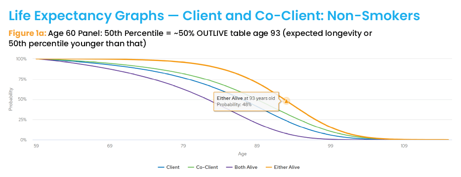
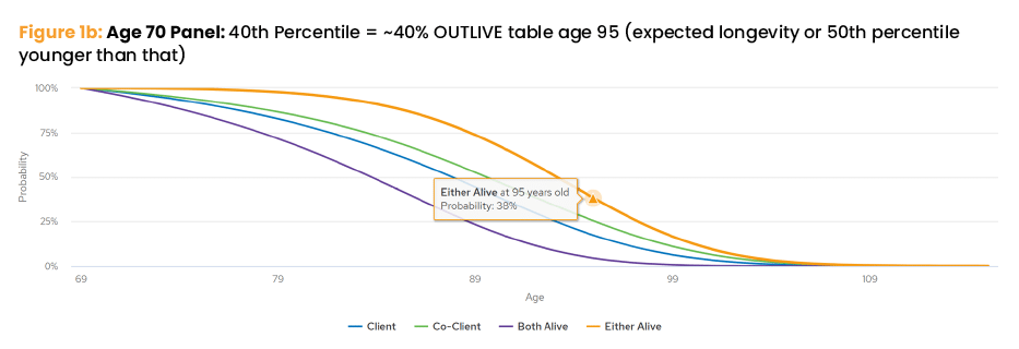
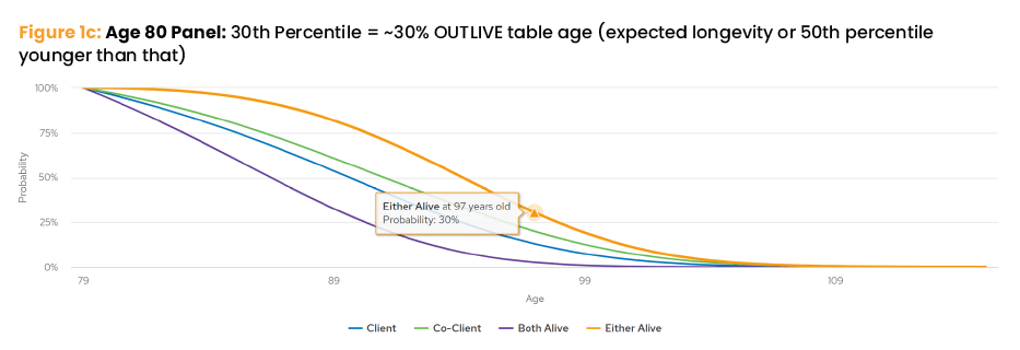
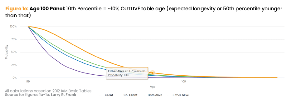
The series of graphs that are part of Figure 1 illustrate how you can use Money Guide Pro’s calculator in a more nuanced manner to help clients.
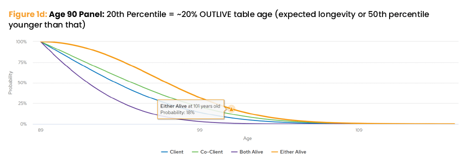
Let’s start with Figure 1a. It shows that for a non-smoking couple, now both 60 years old, there is a 48% probability that either spouse will live beyond age 93. So, the remaining time period for income calculations is 33 years (93 minus 60). However, now look at Figure 1d. If either of them is still alive at age 90, his or her remaining time-period for income calculations is now just 11 years (101 minus 90). Consider that 18% of 90-year-olds outlive age 101 — nowhere near the common 30-year research periods.
The problem is that today’s commonly used static-longevity modeling does not provide much insight into how retirees get from age 60 to 90. Instead, it relies upon expected longevity that, by definition, says that 50% of retirees at any given attained age will outlive their statistical age — which should not be the case at increasingly advanced ages.
Too often, people misinterpret longevity percentages as living to an age. A better interpretation is, what percentage of an age group outlives, or lives past, any longevity age from the tables? How do planners plan for those retirees who continue to live?
For example, Figure 1c shows a 50% probability that either 80-year-old spouse will live past their mid 90s. Based on this, 94 minus 80 equals a 14-year time frame. But the reality is that 30% of today’s 80-year-olds will outlive their expected longevity age of 94 and survive past 97, and nobody knows if they are in that fortunate group. So as retirees age, advisor’s need will better serve clients by slowly extending the time frame that they likely have left to live. At the same time, advisors should recognize that fewer and fewer retirees will reach these later ages and outlive their money. In other words, the traditional expected longevity calculation results a lower drawdown rate for spending than the strategic longevity approach used in the above example.
Figure 1 shows life expectancy at different ages. I’ll explain how to use them in a more effective formula to help clients plan their spending.
The 60 represents the baseline age when many people may begin retirement and 50 represents the 50th percentile — where half the cohort predeceases that age and half outlives that age. Again, this is the definition of expected longevity for each attained age.
Using this model predicts a smaller percentage of cohorts outliving the attained age than traditional models show. Reviewing the SLP each year shows that it becomes less and less likely — barring catastrophic spending — that the retiree will outlive their money. This strategic application is illustrated in the Figure 1 panels.
I went into the logic in more detail in the example above than I do with my retired clients. People intuitively understand that, as they get older, they have less time remaining. However, today’s software does not apply this changing time-frame reality when modeling spending for retiree cash flows and balances. Mindsets are inadvertently fixed to static time frames, not to aging time frames. What people also don’t realize is older retirees have a greater probability of living to more advanced ages than younger retirees. In other words, a 60-year-old has a lower possibility of outliving age 100 (Figure 1a) than a 90-year-old (Figure 1d).
Software today requires advisors to rerun the software in the future to get a spending suggestion in that future. Why not provide better insight today for those future years, too? Failing to, by ignoring the transition to and through the very advanced years, exposes the unintended ageism in the profession. After all, planning is by definition about the future.
Planning needs to be reversed
The current approach to planning (starting with today and looking toward the future) is actually the reverse of how retirement planning should be viewed. It would be better to begin planning for old age and look backward to the present — as shown in Figure 1 where all the time frames are aligned to the end of the longevity table.
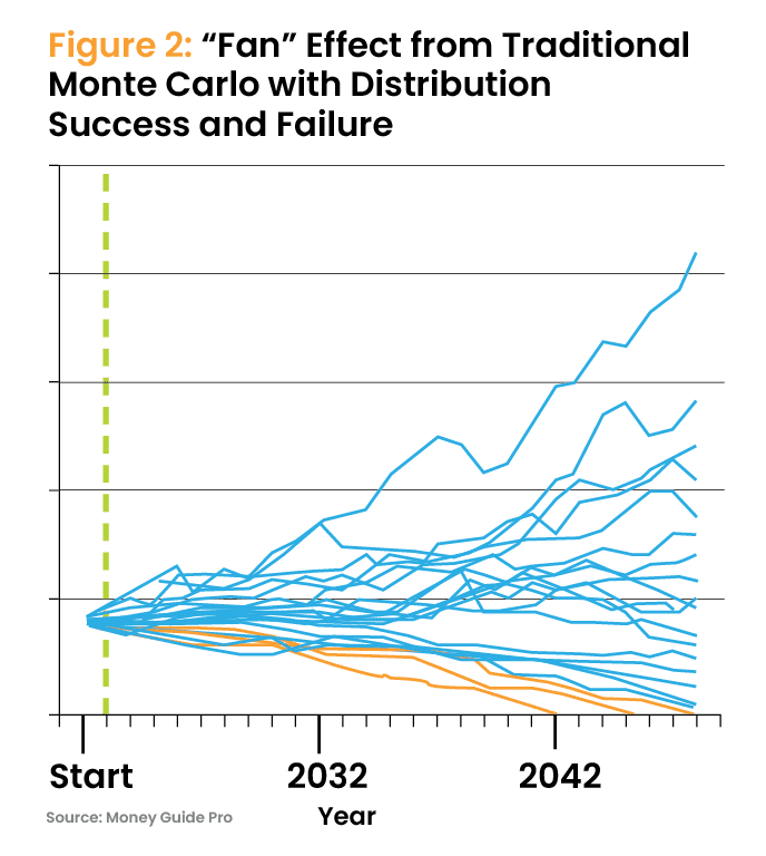
In other words, the question should be, “What is a more realistic cash flow during those older ages?” To me, that is more helpful than saying, “It will probably be between those higher, or lower, amounts” that come from today’s Monte Carlo simulation (Figure 2). But where in between those successes or failures?
Advisors, and retirees, never know which statistical longevity group they may be in, until death informs. But we must assume that retirees who are alive will continue to live, at least for some time. So, why not use statistics rather than today’s “pick an age” approach to plan to?
Some things to consider: Are retirees in the long-lived group, or not? How should planning accommodate this uncertainty? How should modeling slowly transition time periods from longer to shorter to better represent aging effects on portfolio cash flows and balances, which also have their own set of statistical portfolio uncertainty?
Putting it all together
Ageism creeps in when one realizes the statistical effects in the mathematical inputs to the modeling are available, but often given little thought. The exponential effects of aging are always very little in the early time periods and always more pronounced in the later time periods; precisely when those effects are important mathematically for the older retiree.
Using the strategic longevity percentile (SLP) model, which slowly introduces lower longevity percentiles, instead of the expected longevity model, can smooth out cash-flow adjustments over the entire modeling timeframe. As illustrated in Figure 1, people never reach their expected longevity age because that age always changes as people age! I call this the “Longevity Bow Wave” – a boat never catches the front of its bow wave as long as it keeps moving, and people never catch their expected longevity as long as they are alive.
Clients intuitively understand the bow wave once they see it and then view the income process in a different light since they are less concerned with failure possibilities and more comfortable spending to support their lifestyle at all ages. As retirees age and their life expectancy shrinks, they can spend a higher amount and their drawdown rate can increase because time is shorter. This exponential effect on drawdown rates is not factored into modeling software programs using a static time frame.
Factoring in RMDs
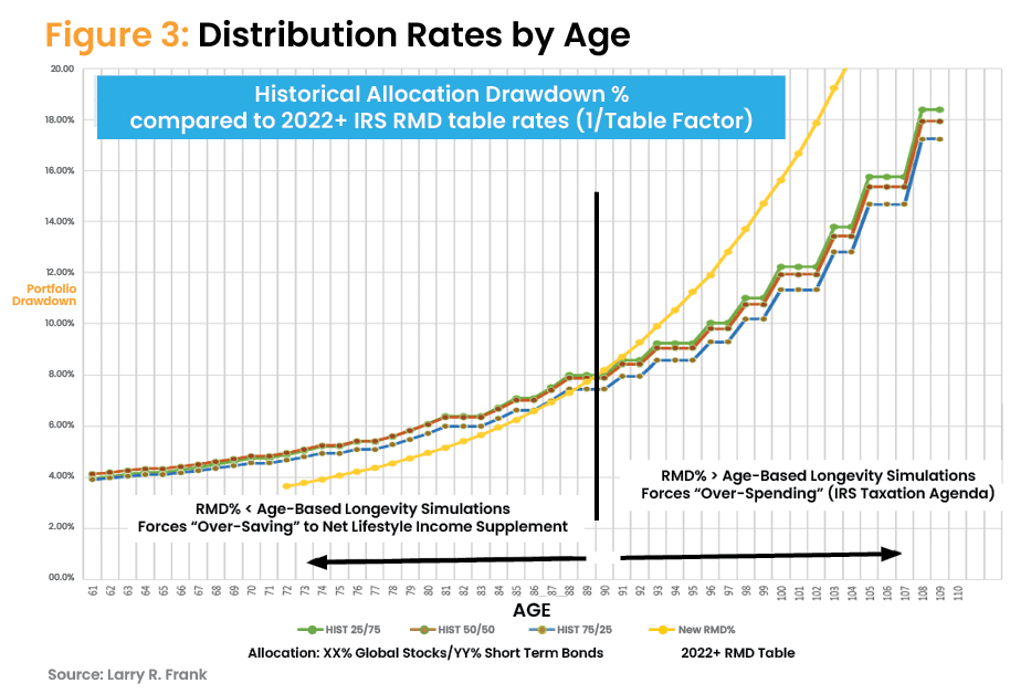
The exponential effect may be seen in Figure 3, which compares the results of the aging process adjustments for three allocations to the IRS’s required minimum distribution (RMD) table. Inverting the factors in the RMD table (1/table factor) converts them to percentages that can be compared to portfolio drawdown percentages by age.
Using the RMD tables relative to an age-based methodology:
Before the crossover point at about age 89, the RMD tables tend to underestimate what people can safely spend.Younger retirees either spend less using the RMD tables or are forced to save more to fund the lifestyle suggested by the age-based method. For example, let’s say the RMD table factor for a 75-year-old is 24.6. The inverse (1/24.6) equals 4.06%. So for every $100,000 the client may have, that would be $4,060. Let’s say the age-based drawdown rate is 5.25%, or $5,250. The RMD method would require this 75-year-old to have saved $129,310 to withdraw the $5,250 (129,310 x 4.06%) to support their target lifestyle standard of living. In other words, spend less or save more.
After the crossover point, retirees are forced to withdraw more (though they need to pay taxes and don’t need to spend it all). In other words, RMDs encourage retirees to spend more, relative to reinvesting some of the RMD (after taxes) back into their portfolio to retain money so they don’t outlive their money as they continue to age.
Always remember the “longevity bow wave” effect. For example, the RMD table rate for a 95-year-old may be 8.9, and the inverse (1/8.9) equals 11.2%. For every $100,000 they may have, that would be $11,200. The age-based drawdown rate is 9.3%, or $9,300. The RMD method requires this retiree to withdraw an extra $1,900 per $100,000 over their target lifestyle standard of living — maybe even more since research shows older retirees spend less than their younger years.
Although this example appears small, note in Figure 3 that the excess grows as the retiree ages. That excess should be reinvested to ensure they don’t outlive their money by continuing to live (a form of saving “personal mortality credits”). Software should suggest how much retirees should save relative to their desired lifestyle. I tell clients they can spend slightly more money when they are more active.
The RMD tables do account for longevity adjustments. However, from the examples above, longevity alone does not account for the exponential effect coming from ever-shorter time periods from aging.
Muting the impact
The exponential effect may be muted by applying a simple adjustment to a drawdown rate each year. Here’s the formula:
Applying mathematically 1 – 1/n, where n is the number of years in each simulation time-period for each age, mutes the exponentiality seen in the RMD tables and today’s software programming. This exponentiality comes from ever shorter time periods as a retiree ages and. picks up rate of change at the end of the time-period, precisely when aging shortens the time frames for portfolio retirement income. Software today does not factor in either shorter time frames or allocation characteristics more appropriate for shorter periods.
Practical application
Strategically applying the longevity timetable frames — rather than using the static-longevity model — and adjusting for the exponentiality that comes from aging can help ensure your clients have portfolio income for as long as they live (again, barring catastrophic spending). These two steps also increase the likelihood that the retiree has bequest balances at all ages; thus, estate planning is also important.
First, determine the number of years the simulation should be cast for each specific retiree from the use of the Strategic Longevity Percentile (SLP) process discussed above. For example, let’s say you arrive at life expectancies of 28 years for a younger retired client and 12 years for an older retired client. You run the simulation for those time periods and obtain the annual spending possible. That annual spending figure divided into the client’s total portfolio value is the drawdown rate.
For example, you determine the drawdown rates to be 5.75% for the younger client and 9.0%, for the older client. The exponential adjusted drawdown rates would be:
Finally, you multiply the exponential adjusted drawdown rate by each retiree’s total portfolio value to arrive at their unique prudent spending levels.
Wouldn’t it be easier if software made these aging adjustments during modeling? I think so.
The evidence
Research demonstrates that portfolio allocation and spend-down time frames (i.e., age) both influence drawdown rates. (Frank, et.al., 2012; Suarez, 2020).
Since retirement income is sensitive to characteristics of both portfolio constitution statistics and longevity statistics, both of which vary ever so slightly over time, solving for income over time (i.e., aging) becomes similar to a problem that can be solved using algebra.
Today’s software takes a single time period, with single portfolio characteristics, and uses this to calculate necessary income throughout a retiree’s lifetime. Yet, we know this information is not fixed over that timeframe. Instead, software should be programmed to also suggest what portfolio allocation should be applied at what ages. In other words, what allocation should be solved for now? And at what age should that allocation be changed to correspond to shorter expected time frames?
4% shortcomings
William Bengen published his seminal work that ultimately transitioned advisor thinking from rote method planning to stochastic Monte Carlo modeling. The 4% rule emerged from Bengen’s work and assumes 30 years in retirement. But like shortfalls of the RMD rule noted above, the 4% rule also ignores the shorter periods that Bengen researched and is another example of unintended ageism bias of the profession.
The 4% rule originated almost 30 years ago. How much have hardware and software programming evolved over the past 30 years? How much of that evolved progress has made its way into retirement income planning software and thought?
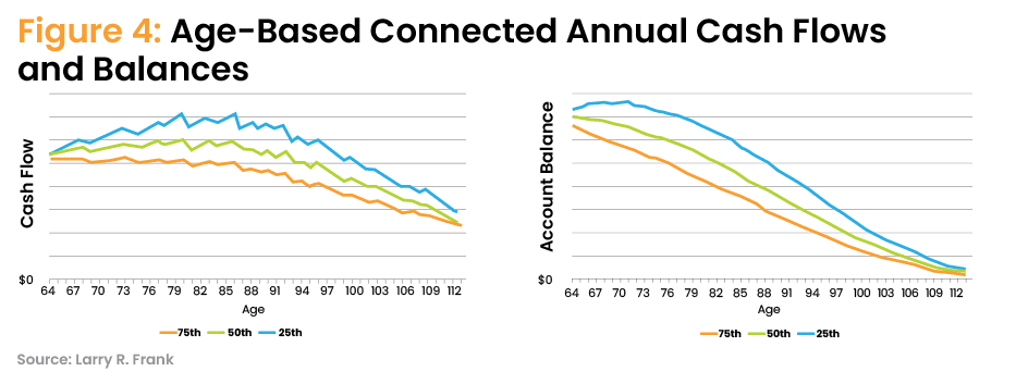
Also, old school is the way Monte Carlo simulations are run to model aging. Monte Carlo projections represent ever growing uncertainty in the future (the “fan” effect, shown in Figure 2). Contrast Figure 2 with a modernized use of time frames representing aging that strategically focus rolling Monte Carlo cash flows and balances into a narrower range of uncertainty (Figure 4) and a better understanding of bequests. Figure 4 illustrates unconstrained spending. If the retiree sets a spending ceiling (spend “no more than” $X per month), or spending floor (spend “no less than” $Y), then the tail ends of the balances graph shifts up or down, respectively. Such discussion is beyond the scope of this introductory article, though you may intuitively understand those outcomes.
Looking ahead
Most advisors intuitively know longevity expectations change with age and that modeling income is not one-and-done. Knowing these subtleties, they should ask for better software that models cash flows and balances to better simulate the aging process’s effects on future cash flows and portfolio balances. Such software would move the profession’s unintended ageism against clients to the past.
My clients appreciate the understanding that their modeling continues as long as they live, regardless of their current age
Why isn’t software programmed to model our intuition, rather than perform single period/single allocation calculations? Income Lab is relatively new software that comes closest to managing retiree spending with rolling longevity, as well as flexible spending on the margins, in mind.
1Frank, Larry R. 2022. “What are the Three Paradigms of Retirement Income Planning?” Journal of Economics, Finance and Management Studies.5 (4): 700-720.
Larry R. Frank Sr., MBA, CFP, founder/owner Better Financial Education and a registered investment advisor and researcher. He has been advising clients for 30 years and has published 10 academic research papers in various journals. To contact him or see his research, visit him on LinkedIn.